파이토치 기초 정리
파이토치 기초
파이토치(Pytorch)는 페이스북에서 루아(Lua)언어로 개발된 토치(Torch)를 파이썬 버전으로 개발한 딥러닝 라이브러리로, 과학 연산을 위한 라이브러리로 초기에 공개되었다. 이후 GPU를 이용한 텐서 조작, 동적 신경망 구축이 가능하도록 딥러닝 프레임워크로 발전시키고 있다. 파이토치는 넘파이(Numpy)와 유사하지만, 유연하면서도 가속화된 계산 속도를 제공한다. 파이토치의 구성요소는 torch, torch.autograd, torch.nn, torch.multiprocessing, torch.optim, torch.utils, torch.onnx 등이 있으며 기본 데이터 표현을 위해 텐서(tensor)를 사용한다. 텐서는 일반적으로 수치형 데이터를 저장하는 컨테이너이며 GPU를 사용한 연산 가속도 가능하다. 텐서는 비어있는 텐서, 랜덤으로 초기화된 텐서, 데이터 타입이 long이고 0으로 채워진 텐서, 사용자가 입력한 값으로 초기화된 텐서, x와 같은 크기이면서 float 타입이고 무작위로 채워진 텐서 등 여러가지로 생성할 수 있다. 텐서의 크기는 torch.Size로 계산할 수 있고, 데이터 타입은 FloatTensor, IntTensor 등으로 다양하다
아래는 파이토치(Pytorch)로 컨볼루션 신경망을 만드는 코드 예시이다.
# 입력 데이터를 확인하기 위한 변수 생성
import torch
import torch.nn as nn

# 컨볼루션 신경망 구조 생성
class CNN(nn.Module):
    def __init__(self):
        super(CNN, self).__init__()
        self.layer1 = nn.Sequential(
            nn.Conv2d(1, 16, kernel_size=5, padding=2),
            nn.BatchNorm2d(16),
            nn.ReLU(),
            nn.MaxPool2d(2))
        self.layer2 = nn.Sequential(
            nn.Conv2d(16, 32, kernel_size=5, padding=2),
            nn.BatchNorm2d(32),
            nn.ReLU(),
            nn.MaxPool2d(2))
        self.fc = nn.Linear(7*7*32, 10)

    def forward(self, x):
        out = self.layer1(x)
        out = self.layer2(out)
        out = out.view(out.size(0), -1)
        out = self.fc(out)
        return out

cnn = CNN()
파이토치의 구성요소
torch : 메인 네임스페이스, 텐서 등의 다양한 수학 함수가 포함 torch.autograd : 자동 미분기능을 제공하는 라이브러리 torch.nn : 신경망 구축을 위한 데이터 구조나 레이어 등의 라이브러리 torch.multiprocessing : 병렬처리 기능을 제공하는 라이브러리 torch.optim : SGD(Stochastic Gradient Descent)를 중심으로 한 파라미터 최적화 알고리즘 제공 torch.utils : 데이터 조작 등 유틸리티 기능 제공 torch.onnx : ONNX(Open Neural Network Exchange), 서로 다른 프레임워크 간의 모델을 공유할 때 사용
텐서(Tensor)
데이터표현을 위한 기본 구조로 텐서(tensor)를 사용 텐서는 데이터를 담기 위한 컨테이너(container)로서 일반적으로 수치형 데이터를 저장 넘파이(Numpy)의 ndarray와 유사 GPU를 사용한 연산 가속 가능
텐서 초기화와 데이터 타입
초기화 되지 않은 텐서
import torch

x = torch.empty(4, 2)
print(x)
torch에 비어있는 텐서를 생성
무작위로 초기화된 텐서
x = torch.rand(4, 2)
print(x)
랜덤을 기준으로 초기화가 된 텐서
데이터 타입(dtype)이 long이고, 0으로 채워진 텐서
x = torch.zeros(4, 2, dtype=torch.long)
print(x)
데이터 타입이 long이면서 0으로 채워진 텐서를 생성 long타입이기 때문에 소수점없이 정수인 상태로 생성
사용자가 입력한 값으로 텐서 초기화
x = torch.tensor([3, 2.3])
print(x)
2 x 4, double 타입, 1로 채워진 텐서
x = torch.ones(2, 4, dtype=torch.double)
print(x)
2 x 4 크기의 1로 채워진 텐서 생성
x와 같은 크기, float 타입, 무작위로 채워진 텐서
x = torch.ones(2, 4, dtype=torch.double)
x = torch.randn_like(x, dtype=torch.float)
print(x)
torch.randn_like를 통해 그 전의 x와 같은 모양의 텐서를 생성 그러나 데이터 타입은 float
텐서의 크기 계산
x = torch.ones(2, 4, dtype=torch.double)
print(x.size())
데이터 타입(Data Type)
Data type dtype CPU tensor GPU tensor
| 32-bit floating point | torch.float32 or torch.float | torch.FloatTensor | torch.cuda.FloatTensot |
| 64-bit floating point | torch.float64 or torch.double | torch.DoubleTensor | torch.cuda.DoubleTensor |
| 16-bit floating point | torch.float16 or torch.half | torch.HalfTensor | torch.cuda.HalfTensor |
| 8-bit integer(unsinged) | torch.uint8 | torch.ByteTensor | torch.cuda.ByteTensor |
| 8-bit integer(singed) | torch.int8 | torch.CharTensor | torch.cuda.CharTensor |
| 16-bit integer(singed) | torch.int16 or torch.short | torch.ShortTensor | torch.cuda.ShortTensor |
| 32-bit integer(singed) | torch.int32 or torch.int | torch.IntTensor | torch.cuda.IntTensor |
| 64-bit integer(singed) | torch.int64 or torch.long | torch.LongTensor | torch.cuda.LongTensor |
ft = torch.FloatTensor([1, 2, 3])
print(ft)
print(ft.dtype)
print(ft.short())
print(ft.int())
print(ft.long())

it = torch.IntTensor([1, 2, 3])
print(it)
print(it.dtype)
print(it.float())
print(it.double())
print(it.half())
CUDA Tensors
x = torch.randn(1)
print(x)
print(x.item())
print(x.dtype)

device = torch.device('cuda' if torch.cuda.is_available() else 'cpu')
print(device)
y = torch.ones_like(x, device=device)
print(y)
x = x.to(device)
print(x)
z = x + y
print(z)
print(z.to('cpu', torch.double))
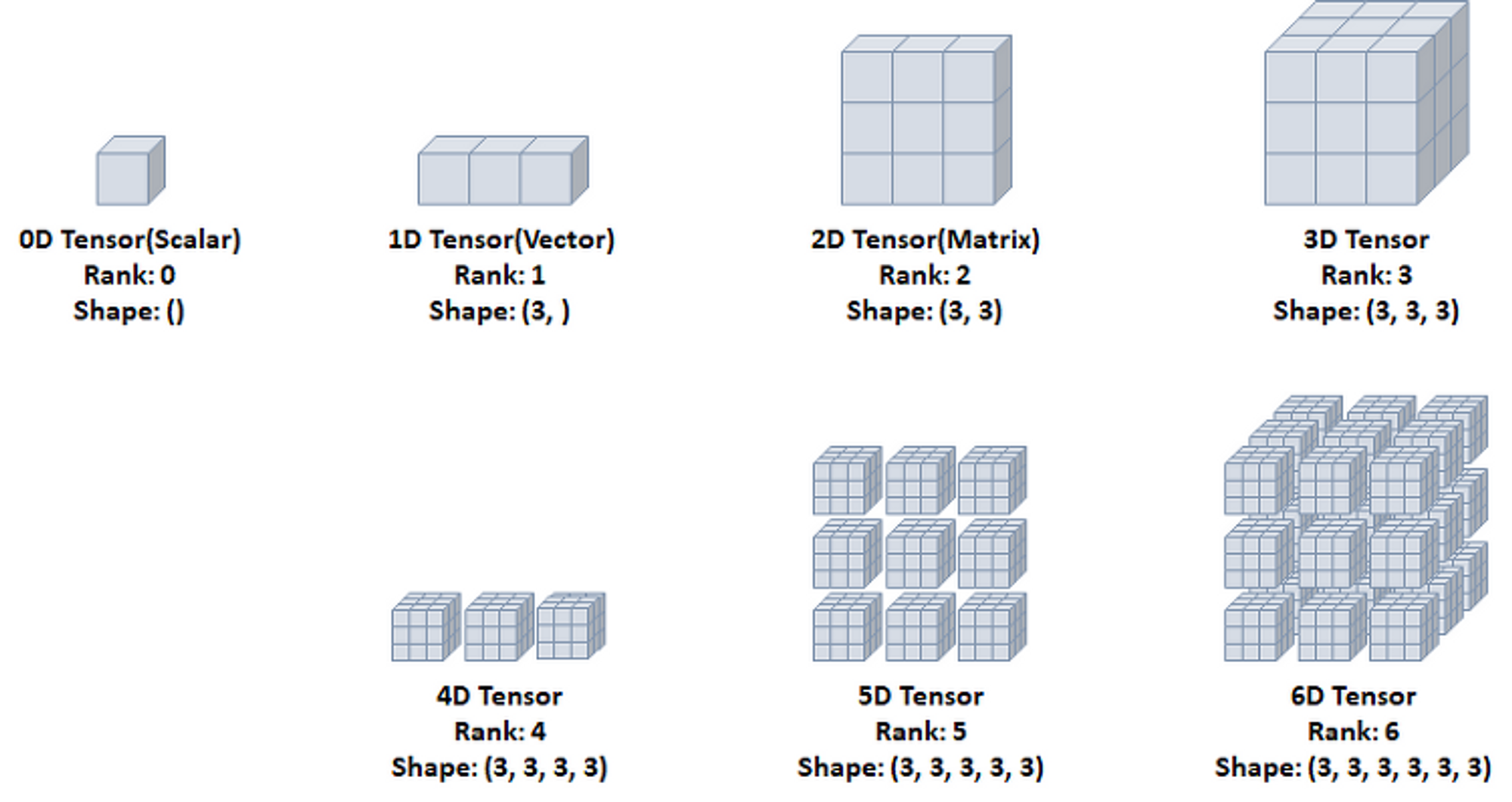
다차원 텐서 표현
0D Tensor(Scalar)
- 하나의 숫자를 담고 있는 텐서(Tensor)
- 축과 형상이 없음
t0 = torch.tensor(0)
print(t0.ndim)
print(t0.shape)
print(t0)
1D Tensor(Vector)
- 값들을 저장한 리스트와 유사한 텐서
- 하나의 축이 존재
t1 = torch.tensor([1, 2, 3])
print(t1.ndim)
print(t1.shape)
print(t1)
2D Tensor(Matrix)
- 행렬과 같은 모양으로 두개의 축이 존재
- 일반적인 수치, 통계 데이터셋이 해당
- 주로 샘플(samples)과 특성(features)을 가진 구조로 사용
t2 = torch.tensor([[1, 2, 3],
                  [4, 5, 6],
                  [7, 8, 9]])
print(t2.ndim)
print(t2.shape)
print(t2)
3D Tensor
- 큐브(cube)와 같은 모양으로 세개의 축이 존재
- 데이터가 연속된 시퀀스 데이터나 시간 축이 포함된 시계열 데이터에 해당
- 주식 가격 데이터셋, 시간에 따른 질병 발병 데이터 등이 존재
- 주로 샘플(samples), 타임스텝(timesteps), 특성(features)을 가진 구조로 사용
t3 = torch.tensor([[[1, 2, 3],
                    [4, 5, 6],
                    [7, 8, 9],
                    [1, 2, 3],
                    [4, 5, 6],
                    [7, 8, 9]]])
print(t3.ndim)
print(t3.shape)
print(t3)
4D Tensor
- 4개의 축
- 컬러 이미지 데이터가 대표적인 사례 (흑백 이미지 데이터는 3D Tensor로 가능)
- 주로 샘플(samples), 높이(height), 너비(width), 컬러 채널(channel)을 가진 구조로 사용
5D Tensor
- 5개의 축
- 비디어 데이터가 대표적인 사례
- 주로 샘플(samples), 프레임(frames), 높이(height), 너비(width), 컬러 채널(channel)을 가진 구조로 사용
텐서의 연산(Operations)
텐서에 대한 수학 연산, 삼각함수, 비트 연산, 비교 연산, 집계 등 제공
a = torch.rand(1, 2) * 2 - 1
print(a)
print(torch.abs(a))
print(torch.ceil(a))
print(torch.floor(a))
print(torch.clamp(a, -0.5, 0.5))
a = torch.rand(1, 2) * 2 - 1

print(a)
print(torch.min(a))
print(torch.max(a))
print(torch.mean(a))
print(torch.std(a))
print(torch.prod(a))
print(torch.unique(torch.tensor([1, 2, 3, 1, 2, 2])))
max와 min은 dim 인자를 줄 경우 argmax와 argmin도 함께 리턴
- argmax : 최대값을 가진 인덱스
- argmin : 최소값을 가진 인덱스
x = torch.rand(2, 2)
print(x)
print(x.max(dim=0))
print(x.max(dim=1))
dim = 0 일 때 열로 가면서 위 아래를 비교 dim = 1 일 때 행으로 가면서 좌우를 비교
사칙연산 : torch.add, sub, mul, div
x = torch.rand(2, 2)
print(x)
y = torch.rand(2, 2)
print(y)

print(x + y)
print(torch.add(x, y))

print(x - y)
print(torch.sub(x, y))
print(x.sub(y))

print(x * y)
print(torch.mul(x, y))
print(x.mul(y))

print(x / y)
print(torch.div(x, y))
print(x.div(y))
결과 텐서를 인자로 제공
x = torch.rand(2, 2)
print(x)
y = torch.rand(2, 2)
print(y)

result = torch.empty(2, 4)
torch.add(x, y, out=result)
print(result)
x 와 y를 더해주기, 결과는 result에 저장하기
in-place 방식
in-place 방식으로 텐서의 값을 변경하는 연산 뒤에는 _가 붙음
x = torch.rand(2, 2)
print(x)
y = torch.rand(2, 2)
print(y)

y.add_(x)
print(y)
in-place 방식은 텐서의 값을 변경한 다음에 변경하는 연산 자체에 _를 붙임. 복사를 하는 것
y의 값에 x의 값을 더한 값을 y에 저장해줌.
내적(dot product) : torch.mm
x = torch.rand(2, 2)
print(x)
y = torch.rand(2, 2)
print(y)

print(torch.matmul(x, y))
z = torch.mm(x, y)
print(z)
print(torch.svd(z))
텐서의 조작(Manipulations)
인덱싱(Indexing): Numpy처럼 인덱싱 형태로 사용가능
x = torch.Tensor([[1, 2],
                  [3, 4]])

print(x)
print(x[0, 0])
print(x[0, 1])
print(x[1, 0])
print(x[1, 1])
print(x[:, 0])
print(x[:, 1])
view() : 텐서의 크기(size)나 모양(shape)을 변경
- 기본적으로 변경 전과 후에 텐서 안의 원소 개수가 유지되어야 함
- 1로 설정되면 계산을 통해 해당 크기값을 유추
x = torch.randn(4, 5)
print(x)
y = x.view(20)
print(y)
z = x.view(5, -1)
print(z)
item: 텐서에 값이 단 하나라도 존재하면 숫자값을 얻을 수 있음
x = torch.randn(1)
print(x)
print(x.item())
print(x.dtype)
스칼라값 하나만 존재해야 item() 사용 가능
squeeze : 차원을 축소(제거)
x = torch.randn(1, 3, 3)
print(x)
print(x.shape)

y = x.squeeze()
print(y)
print(y.shape)
unsqueeze : 차원을 증가(생성)
x = torch.randn(3, 3)
print(x)
print(x.shape)

y = x.unsqueeze(dim=0)
print(y)
print(y.shape)
stack : 텐서간 결합
x = torch.FloatTensor([1, 4])
print(x)
y = torch.FloatTensor([2, 5])
print(y)
z = torch.FloatTensor([3, 6])
print(z)

print(torch.stack([x, y, z]))
cat : 텐서를 결합하는 메소드(concatenate)
- 넘파이의 stack와 유사하지만, 쌓을 dim이 존재해야함
- 해당 차원을 늘려준 후 결합
a = torch.randn(1, 3, 3)
print(a)
b = torch.randn(1, 3, 3)
print(b)

c = torch.cat((a, b), dim=0)
print(c)
print(c.size())
chunk: 텐서를 여러 개로 나눌 때 사용 (몇 개로 나눌 것인가?)
a = torch.randn(3, 6)
print(a)
t1, t2, t3 = torch.chunk(a, 3, dim=1)
print(t1)
print(t2)
print(t3)
t1, t2, t3 = a를 3개로 나눠줘. dim=1로 (진행방향 열→)
split: chunk와 동일한 기능이지만 조금 다름(텐서의 크기는 몇인가?)
a = torch.randn(3, 6)
print(a)
t1, t2, t3 = torch.split(a, 2, dim=1)
print(t1)
print(t2)
print(t3)
torch ↔ numpy
- Torch Tensor(텐서)를 Numpy array(배열)로 변환가능
- numpy()
- from_numpy()
- Tensor가 CPU상에 있다면 Numpy 배열은 메모리 공간을 고유하므로 하나가 변하면, 다른 하나도 변함.
a = torch.ones(7)
print(a)

b = a.numpy()
print(b)

a.add_(1)
print(a)
print(b)
a에 값에 1을 더해줬는데 b도 2가 출력됨. 텐서가 cpu상에 있으면 메모리 공간을 공유함.
a = np.ones(7)
b = torch.from_numpy(a)
np.add(a, 1, out=a)
print(a)
print(b)
a에 numpy로 선언. b에 a를 토치형태로 바꿈 a에 1을 더해주고 그 값을 a에 넣어준다. b의 값도 2가 됨.
Autograd(자동미분)
- torch.autograd 패키지는 Tensor의 모든 연산에 대해 자동 미분 제공
- 코드를 어떻게 작성하여 실행하느냐에 따라 역전파가 정의됨.
- backprop를 위해 미분값을 자동으로 계산
requires_grad속성을 True로 설정하면, 해당 텐서에서 이루어지는 모든 연산들을 추적하기 시작. 기록을 추적하는 것을 중단하게 하려면, .detach()를 호출하여 연산기록으로부터 분리
a = torch.randn(3, 3)
a = a * 3
print(a)
print(a.requires_grad)

a.requires_grad_(True)
print(a.requires_grad)

b = (a * a).sum()
print(b)
print(b.grad_fn)
기본적으로는 텐서가 grad를 False로 가지고 있음
requires_grad_(…)는 기존 텐서의 requires_grad값을 바꿔치기(in_place)하여 변경 grad_fn : 미분값을 계산한 함수에 대한 정보 저장 (어떤 함수에 대해서 backprop 했는지)
x = torch.ones(3, 3, requires_grad=True)  # 추적할 수 있게 True
print(x)

y = x + 5
print(y)

z = y * y
out = z.mean()
print(z, out)
계산이 완료된 후, .backward()를 호출하면 자동으로 역전파 계산이 가능하고, .grad속성에 누적됨
x = torch.ones(3, 3, requires_grad=True)  # 추적할 수 있게 True
y = x + 5
z = y * y
out = z.mean()

print(out)
out.backward()
grad : data가 거쳐온 layer에 대한 미분값 저장
x = torch.ones(3, 3, requires_grad=True)  # 추적할 수 있게 True
y = x + 5
z = y * y
out = z.mean()
out.backward()

print(x)  # x 값은 (3, 3) 1로 들어가 있
print(x.grad)  # grad를 통해 미분값을 알려달라고 함.
x = torch.randn(3, requires_grad=True)
y = x * 2
while y.data.norm() < 1000:
    y = y * 2
print(y)

v = torch.tensor([0.1, 1.0, 0.0001], dtype=torch.float)
y.backward(v)  # v기준으로 backward가 됨. -> 0.1, 1.0, 0.0001 기준으로 3개에 대해서 계산이 됨
print(x.grad)
with torch.no_grad()를 사용하여 기울기의 업데이트를 하지 않음
기록을 추적하는 것을 방지하기 위해 코드 블럭을 with torch.no_grad()로 감싸면 기울기 계산은 필요없지만, requires_grad=True로 설정되어 학습 가능한 매개변수를 갖는 모델을 평가(evaluate)할 때 유용
x = torch.randn(3, requires_grad=True)
y = x * 2
while y.data.norm() < 1000:
    y = y * 2

v = torch.tensor([0.1, 1.0, 0.0001], dtype=torch.float)
y.backward(v)  # v기준으로 backward가 됨. -> 0.1, 1.0, 0.0001 기준으로 3개에 대해서 계산이 됨
print(x.requires_grad)
print((x ** 2).requires_grad)

with torch.no_grad():
    print((x ** 2).requires_grad)
detach(): 내용물(content)은 같지만 requires_grad가 다른 새로운 Tensor를 가져올 때
x = torch.randn(3, requires_grad=True)
y = x * 2
while y.data.norm() < 1000:
    y = y * 2

v = torch.tensor([0.1, 1.0, 0.0001], dtype=torch.float)
y.backward(v)
print(x.requires_grad)
y = x.detach()
print(y.requires_grad)
print(x.eq(y).all())  # y랑 x랑 같냐?
자동 미분 흐름 예제
계산 흐름 a → b → c → out backward()를 통해 a ← b ← c ← out 을 계산하면 $\partial out \over \partial a$이 a.grad에 채워짐
a = torch.ones(2, 2)
print(a)

a = torch.ones(2, 2, requires_grad=True)
print(a)

print(a.data)
print(a.grad)
print(a.grad_fn)
a = torch.ones(2, 2, requires_grad=True)
b = a + 2
c = b ** 2
out = c.sum()
out.backward()

print(a.data)
print(a.grad)
print(a.grad_fn)
- a.data, a.grad, a.grad_fn
- tensor([[1., 1.], [1., 1.]]) tensor([[6., 6.], [6., 6.]]) # None # tensor a는 a자체를 직접적으로 계산한 것은 없음 # a의 값을 활용했을 뿐 a의 값에서 뭔가 반영이 된 것은 없기 때문
- b.data, b.grad, b.grad_fn
- tensor([[3., 3.], [3., 3.]]) None <AddBackward0 object at 0x00000202EA7E5B20>
- c.data, c.grad, c.grad_fn
- tensor([[9., 9.], [9., 9.]]) None <PowBackward0 object at 0x000002753FD05B20>
- out.data, out.grad, out.grad_fn
- tensor(36.) None <SumBackward0 object at 0x000001E4F30A5B20>
데이터 준비
파이토치에서는 데이터 준비를 위해 torch.utils.data의 Dataset과 DataLoader사용 가능
Dataset에는 다양한 데이터셋 존재
DataLoader와 Dataset을 통해 batch_size, train 여부, transform 등을 인자로 넣어 데이터를 어떻게 load할 것인지 정해줄 수 있음.
텐서의 구체적인 형태는 size()함수 또는 shape를 사용하여 각 차원의 크기를 확인할 수 있음.
단순히 텐서의 랭크를 확인하려면 ndimension() 함수를 사용하여 알 수 있음.
print('Size:', x.size())
print('Shape:', x.shape)
print('랭크(차원):', x.ndimension())
unsqueeze(), squeeze(), view() 함수로 텐서의 랭크와 shape를 인위적으로 바꿀 수 있다.
# 랭크 늘리기

x = torch.tensor([[1, 2, 3], [4, 5, 6], [7, 8, 9]])
x = torch.unsqueeze(x, 0)
print(x)
print('Size:', x.size())
print('Shape:', x.shape)
print('랭크(차원):', x.ndimension())
[3, 3] 형태의 랭크 2 텐서의 첫 번째(0번째) 자리에 1이라는 차원 값을 추가해 [1, 3, 3] 모양의 랭크 3텐서로 변경한다. 이 때 랭크는 늘어나도 텐서 속 원소의 수는 유지된다.
squeeze() 함수를 이용하면 텐서의 랭크 중 크기가 1인 랭크를 삭제하여 다시 랭크 2 텐서로 되돌릴 수 있다.
[1, 3, 3] → [3, 3] = 크기가 1인 랭크를 삭제
# 랭크 줄이기

x = torch.squeeze(x)
print(x)
print('Size:', x.size())
print('Shape:', x.shape)
print('랭크(차원):', x.ndimension())
view() 함수를 이용하면 직접 텐서의 모양을 바꿀 수 있다.
랭크 2의 [3, 3] 모양 → 랭크 1의 [9]
x = torch.tensor([[1, 2, 3], [4, 5, 6], [7, 8, 9]])
x = x.view(9)

print(x)
print('Size:', x.size())
print('Shape:', x.shape)
print('랭크(차원):', x.ndimension())
squeeze(), unsqueeze(), view() 함수는 텐서의 원소 수를 그대로 유지하면서 모양과 차원을 조절함.
view() 함수로는 텐서의 원소 개수를 바꿀 수는 없음.
view() 함수로 x의 모양이 [2, 4]가 되도록 시도
x = torch.tensor([[1, 2, 3], [4, 5, 6], [7, 8, 9]])

try:
    x = x.view(2, 4)
except Exception as e:
    print(e)
원소가 9개인 텐서를 2 x 4, 원소가 8개인 텐서로는 바꿀 수 없다.
Autograd
w = torch.tensor(1.0, requires_grad=True)

a = w * 3
b = a ** 2
수식으로 표현하면
$$ b = a^2 = (3w)^2 = 9w^2 $$
b를 w로 미분하려면 연쇄법칙을 이용하여 a와 w를 차례대로 미분해야 한다.
backward() 함수를 이용하여 계산 가능
b.backward()
print(f'b를 w로 미분한 값은 {w.grad}')
b에 backward() 함수를 호출함으로써 w.grad는 w가 속한 수식을 w로 미분한 값, 18을 반환한다.
데이터 준비
파이토치에서는 데이터 준비를 위해 torch.utils.data의 Dataset과 DataLoader 사용 가능
Dataset에는 다양한 데이터 셋이 존재